
Projecting a 3D Scene to the Image Plane
26 Feb 2022Given a 3D scene in world coordinates, how does an image of the scene form in the camera, and how do 3D scene points project to the image plane? The short answer to the later question is the camera matrix. And this short note is devoted to deriving the camera matrix. First some mathematical preliminaries.
From Pencils to Points
Consider the generic scenario $\vec{x} \in \mathbb{R}^{n+1}$ and a plane $x_{n+1} = f$. Pencils in $\mathbb{R}^{n+1}$, that is lines which pass through both the origin and $x_{n+1} = f$, map to unique points in plane $x_{n+1} = f$. Figure #1 shows a pencil intersecting plane $x_{n+1} = f$ at unique point $\tilde{x}$.
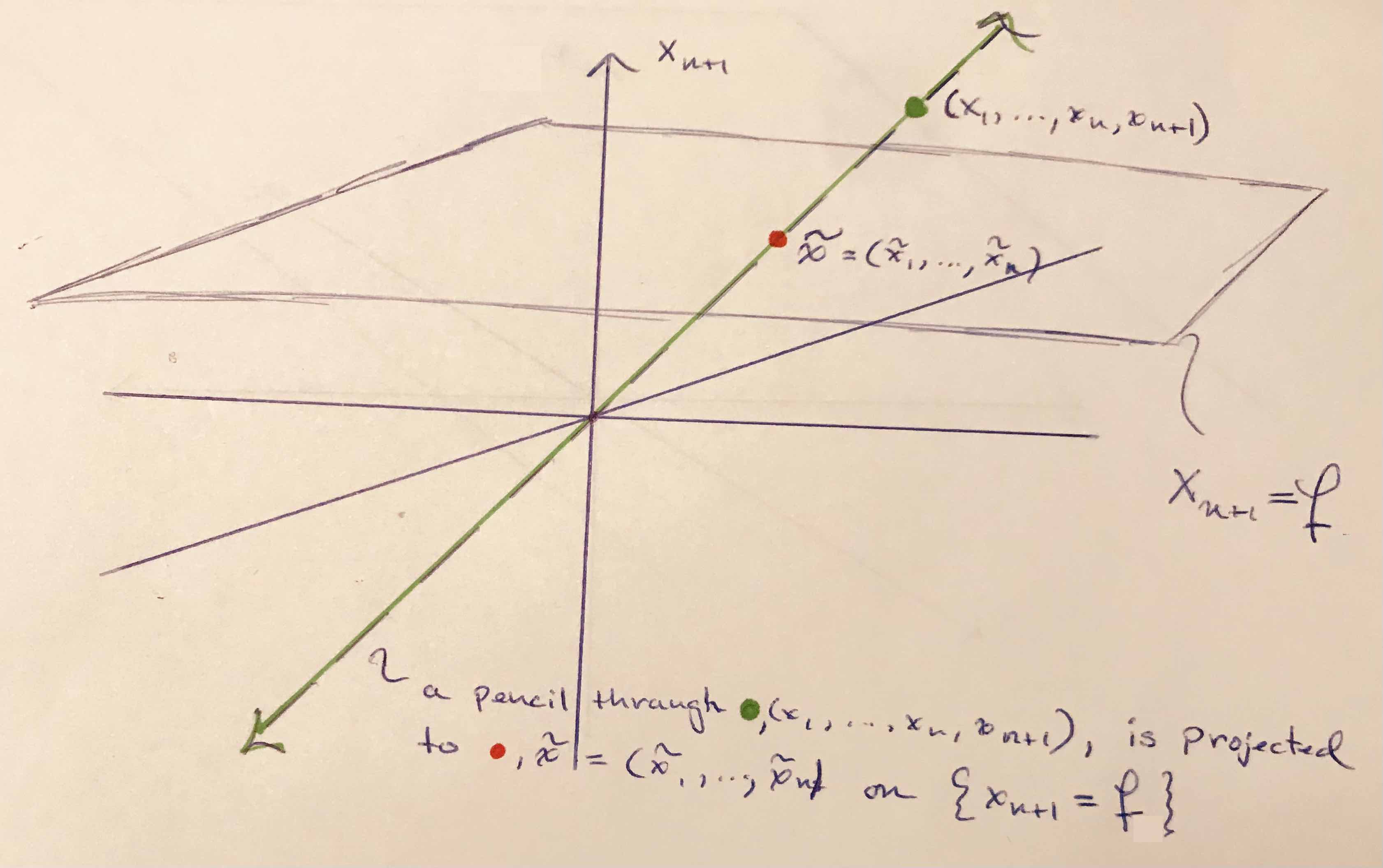
The pencil through $\vec{x} \in \mathbb{R}^{n+1}$ has the form $(tx_1, \cdots, tx_n, tx_{n+1} )$, and it intersects plane $x_{n+1} = f$ when
\[t x_{n+1} = f \quad \Longrightarrow \quad t = \frac{f}{x_{n+1}} .\]The intersection point, the point the line projects to, is described purely as a function of $f$ and $\vec{x}$,
\[\tilde{x} = (f \frac{x_1}{x_{n+1}}, \cdots, f \frac{x_n}{x_{n+1}}) \quad \text{ where } \quad x_{n+1} \neq 0. \\\]The above formula is well defined on pencils. Meaning, given two representatives of a given pencil, say $[a] \sim [b]$, they will both be projected to the same point $\tilde{x}$ in plane $x_{n+1} = f$. Let $K_{n}$ be the projection of $\vec{x} \in \mathbb{R}^{n+1}$ to points on plane $x_{n+1} = f$ and suppose $[a] \sim [b]$, then there is a $t \neq 0$ such that
\[\begin{align} K_n(b) & = (f \frac{b_1}{b_{n+1}}, \cdots, f \frac{b_n}{b_{n+1}}) \\ &= (f \frac{t a_1}{t a_{n+1}}, \cdots, f \frac{t a_n}{t a_{n+1}}) \\ &= K_n(a). \\ \end{align}\]$K_n$ is what’s called a projective transformation because it is well defined on pencils; though sadly, it isn’t also linear because division by $x_{n+1}$ is not. So $K_n$ can’t be expressed in matrix form. However, it can be lifted so that it factors through a projective linear map called $\tilde{K}_n$. To see how break $K_n$ into steps:
- Points are mapped to pencils by the canonical projection $\rho_{n}(\vec{x}) = [\vec{x}] \in \mathbb{RP}^{n}$.
- Pencils are scaled by \(\tilde{K}_n([x_1 : x_2 : \cdots : x_{n+1}]) = [fx_1 : fx_2 : \cdots : fx_n : x_{n+1}]\).
- Project pencils in $\mathbb{R}^{n+1}$ to plane $x_{n+1} = 1$ by $\pi_n([x_1 : x_2 : \cdots : x_{n+1}]) = (\frac{x_1}{x_{n+1}}, \frac{x_2}{x_{n+1}}, \cdots, \frac{x_n}{x_{n+1}})$. Points at infinity are excluded because $x_{n+1} \neq 0$.
Below is a commutative diagram depicting how $K_n$ factors over $\tilde{K}_n$. Recall $\mathbb{R}^{n+1}/{\infty}$ is $\mathbb{R}^{n+1}$ minus points at infinity.
\[% AMScd reference https://www.jmilne.org/not/Mamscd.pdf \begin{CD} \mathbb{RP}^{n} @>\tilde{K_{n}}>> \mathbb{RP}^{n}\\ @A{\rho_n}AA @VV{\pi_n}V \\ \mathbb{R}^{n+1}/\{\infty\} @>{K_n}>> \mathbb{R}^{n} \end{CD}\]$\tilde{K_n}$ does the scaling part of $K_n$, so it is easily written as a projective matrix.
\[\tilde{K_n} = \begin{bmatrix} fI_n & \vec{0} \\ \vec{0} & 1 \\ \end{bmatrix} = \begin{bmatrix} f & & & 0 \\ & \ddots & \Huge0 & \vdots \\ & \Huge0 & f & 0 \\ 0 & \ldots & 0 & 1 \\ \end{bmatrix}. \\\]Applying $\rho_{n}$ and $\tilde{K_n}$ sucessively to $x \in \mathbb{R}^{n+1}$ gives a projective point that $\pi_n$ would project to $\tilde{x}$.
\[\begin{bmatrix} \tilde{x}_1 \\ \vdots \\ \tilde{x}_n \\ 1 \\ \end{bmatrix} \\ {\bf{\Large\sim}} \begin{bmatrix} fx_1 \\ \vdots \\ fx_{n} \\ x_{n+1} \\ \end{bmatrix} \\ = \begin{bmatrix} f & & & 0 \\ & \ddots & \Huge0 & \vdots \\ & \Huge0 & f & 0 \\ 0 & \ldots & 0 & 1 \\ \end{bmatrix} \begin{bmatrix} x_1 \\ x_2 \\ \vdots \\ x_{n+1} \\ \end{bmatrix}. \\\]Pinhole Cameras
A pinhole camera is a simple camera without a lens—effectively a box with a small hole in one side. Light from a scene passes through the hole and projects an inverted image on the opposite side of the box, which is known as the camera obscura effect. A model of the way an image forms in pinhole camera is depicted in Figure #2. Light from points on the tree, for example $x_0$ or $x_1$ in Figure #2, travel along straight lines through the camera center (the blue dot positioned at the origin), and hit the image plane, $f$ units away from the camera center. $f$ is the focal length.
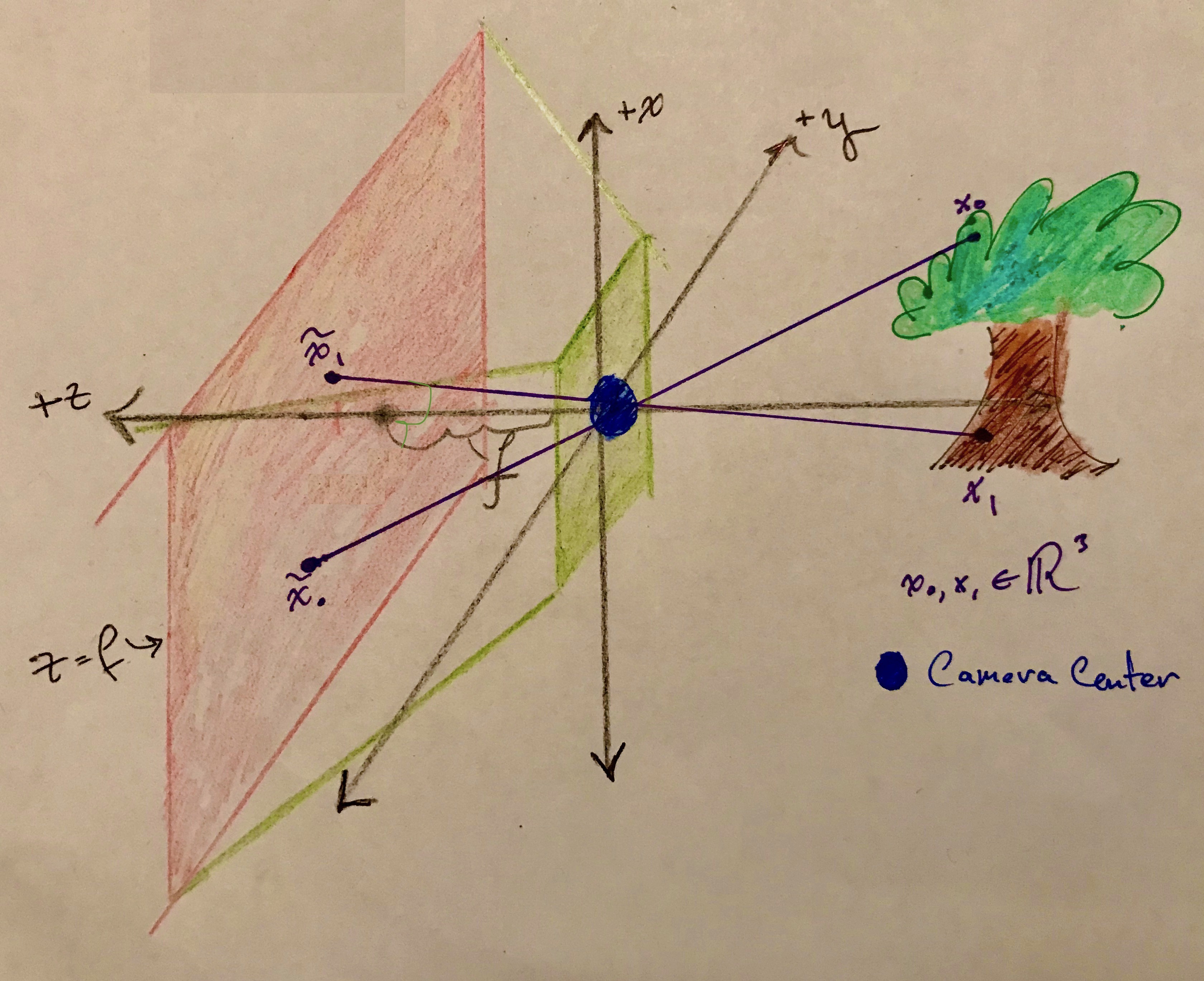
Though not depicted in Figure #2 the tree would be projected on the image plane upside down and flipped about the vertical midline.
The situation depicted in Figure #1 limited to 3D and rotated in the positive $z$ direction $90$ degrees about the $y$-axis also describes image formation – the projection of object points to the image plane. Therefore, the projection of tree points to the image plane is described by projective linear map
\[\tilde{K}_2 =\begin{bmatrix} f & 0 & 0 \\ 0 & f & 0 \\ 0 & 0 & 1 \\ \end{bmatrix} \\ .\]And just like before, applying $\tilde{K}_2$ to tree points gives their corresponding world coordinates on the image plane.
\[\begin{bmatrix} f \frac{x_1}{x_{3}} \\ f \frac{x_2}{x_{3}} \\ 1 \\ \end{bmatrix} \\ {\bf{\Large\sim}} \begin{bmatrix} fx_1 \\ fx_2 \\ x_3 \\ \end{bmatrix} \\ = \begin{bmatrix} f & 0 & 0 \\ 0 & f & 0 \\ 0 & 0 & 1 \\ \end{bmatrix} \\ \begin{bmatrix} x_1 \\ x_2 \\ x_3 \\ \end{bmatrix} \\ .\]From World Coordinates to Camera Coordinates
Projected points $(f\frac{x_1}{x_3}, f\frac{x_2}{x_3}, 1)$ are in the image plane and even span it, however they remain in world coordinates, measured in metric units if the scene is in the real world or some normalized units of a 3D model. By contrast camera coordinates are measured in pixel units. Moreover, the extent of the image plane is actually finite; the film or sensor on which the image is taken is rectangular. A depection of an image senor is shown below in Figure #3. The red rectangle is the image sensor and the ruled elements are pixels. Both $H$ and $W$ are measured in units of the world coordinates, whatever those might be. Without loss of generality assume $H$, $W$, and focal length $f$ are measured in millimeters.
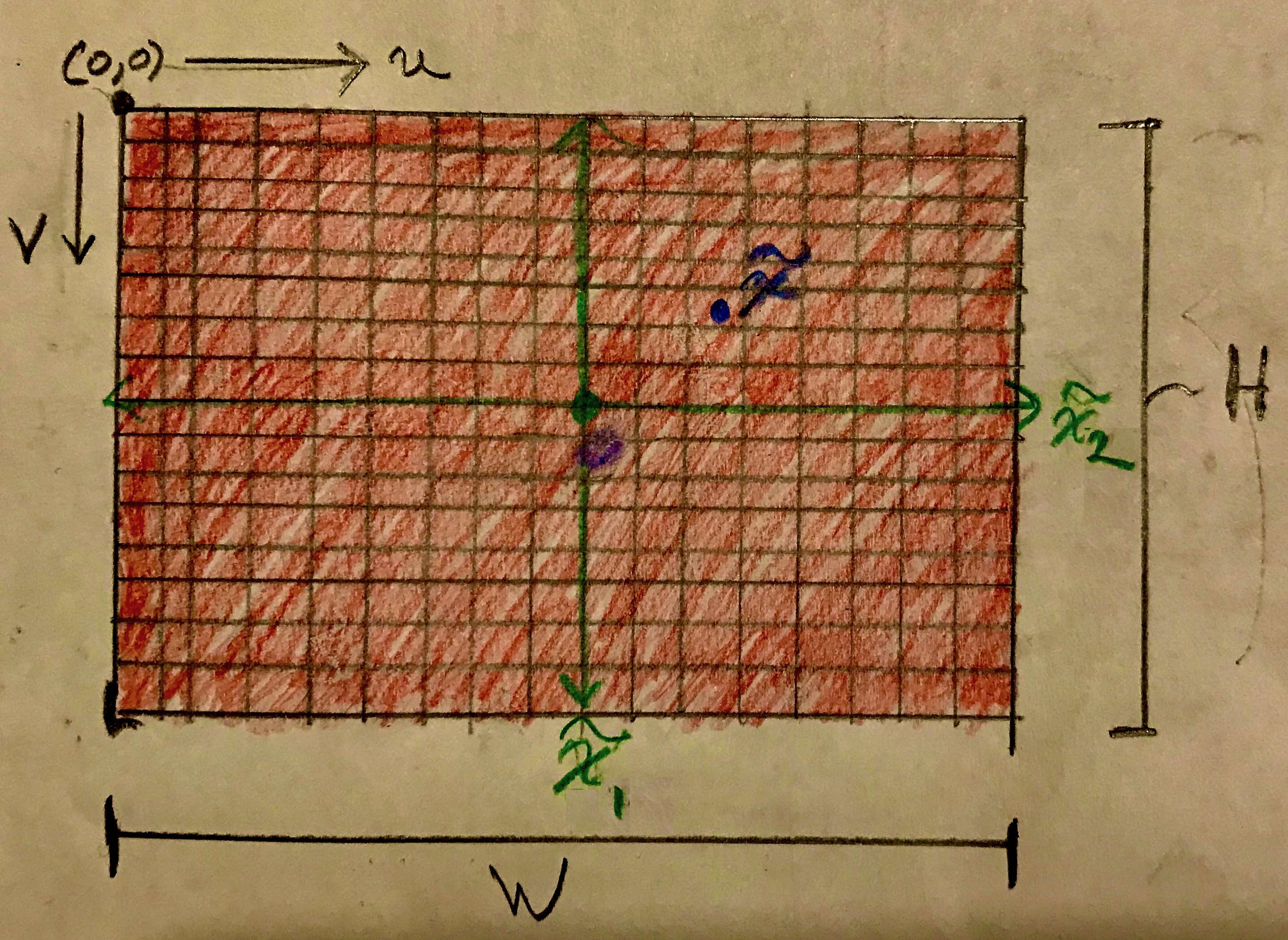
The origin of the camera coordinate system, of the image sensor, is for [odd historical reasons][upper-left] in the upper left corner. Anyhow, it’s nice I suppose that matrices are indexed in the same way. As shown in Figure #3 $(v,u)$ coordinates locate pixels; $v$ is a row index and $u$ is a column index.
Real cameras have lenses and some types of distortion introduced by lenses can be modeled with non-square pixels. While unusual, for the sake of generality I will make the modeling assumption that pixels are rectangular – not necessarily square. Letting the sensor dimensions in pixels be $n \times m$, then the pixel dimensions are $\frac{W}{m}$ mm/pixel in the $u$-direction and $\frac{H}{n}$ in the $v$-direction. Now, to convert points $(f\frac{x_1}{x_3}, f\frac{x_2}{x_3}, 1)$ to pixel units only the focal length $f$ needs to be rescaled because factors $\frac{x_i}{x_3}$ are unitless.
\[\begin{gather} f_u = f \frac{m}{W} \quad \text{and}\quad f_v = f \frac{n}{H} \end{gather}\]are the effective focal lengths in the $u$ & $v$ directions, in pixel units. Having two focal lengths isn’t intuitive, but from the point-of-view of rescaling to pixel units it should be clear. Note that some texts (Solem and Forsyth and Ponce) avoid two focal lengths by choosing a different starting point; namely, $f$ is given in pixels. With no need to convert $f$ to pixels, one would account for non-square pixels by scaling the $u$ coordinate by some calibrated constant $\alpha$, the aspect ratio.
Before continuing a few definitions … Let’s call the coordinate system of points projected to the image plane and converted to pixels, points like $(f_v\frac{x_1}{x_3}, f_u\frac{x_2}{x_3}, 1)$, pixelated coordinates. The green axis in Figure #3 depicts the pixelated coordinate system overlayed onto the image sensor. Define
- optical axis – The line perpendicular to the image plane that passes through the camera center. In Figures #2 and #3 the optical axis is the $x_3$-axis.
- principal point – The point where the optical axis intersects the image plane. It is the origin of the pixelated frame. As depicted in Figure #3, the principal point is typically in the middle of the image plane.
Reindexing Pixelated Coordinates
The goal here is to find a $1$-to-$1$ map $T(p_x,p_y)$ from pixelated coordinates to $(v,u)$ coordinates, while also rectifying the projected image. The image projected on the image plane appears flipped about both the vertical and horizontal midlines. It would be nice to, in one move, reindex and flip the image upright. The left-right inversion/flip is natural and undoing it would result in a mirror image of the object; therfore, to correct the image orientation the projection should only be flipped about its horizontal midline. Figure #4 below depicts a projected image on the image sensor in the pixelated coordinate system; $v$ and $u$ directions are also indicated in the upper left corner. The four corners of the image sensor are labeled with coordinates in the pixelated frame.
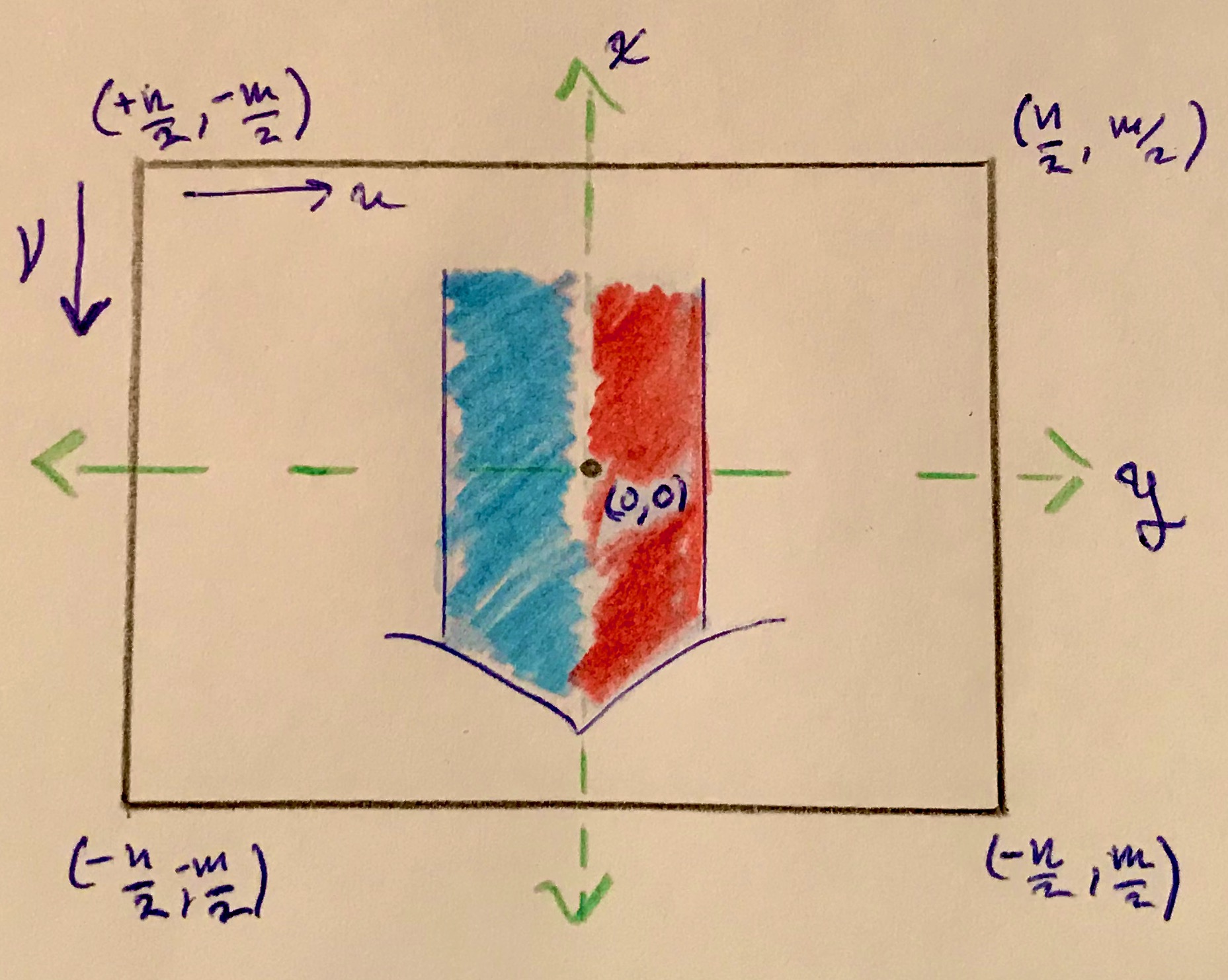
What could the correspondence be? Well, since the middle of the image sensor is the same in both frames, the principal point $(0,0)$ will be mapped to $T(0, 0) = (\frac{n}{2},\frac{m}{2})$. The corners are a different story, because the $(v,u)$ frame is oppositely oriented to the pixelated frame. Notice that while $u$ and $y$ directions have the same orientation (left & right are the same in both frames), $v$ and $x$ point in opposite directions (up in either frame is down in the other). Specifically, this means that the upper left corner of the $(v,u)$ frame is the lower left corner of the pixelated frame. Putting it all together, the corresponding $(v,u)$ coordinates of all four corners are $T(\frac{n}{2},-\frac{m}{2}) = (n,0)$, $T(\frac{n}{2},\frac{m}{2}) = (n,m)$, $T(-\frac{n}{2},\frac{m}{2}) = (0,m)$, and $T(-\frac{n}{2},-\frac{m}{2}) = (0,0)$. These correspondences are also drawn below in Figure #5 in the orientation of the pixelated frame. However, if drawn in the orientation of the $(v,u)$ frame, the result is Figure #6; the image is flipped and is no longer upside down as desired.
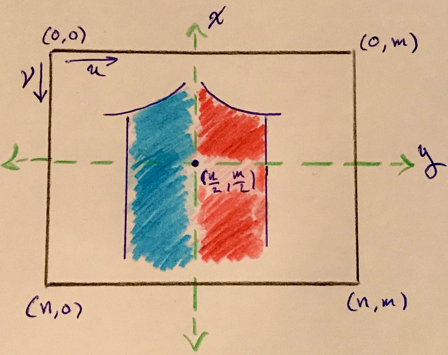
Comparing Figures #4 and #5, one can imagine translating the pixelated frame, into the first quadrant by adding $(\frac{n}{2},\frac{m}{2})$ to each coordinate, $T(p_x, p_y) = (p_x, p_y) + (\frac{n}{2},\frac{m}{2})$. Amazingly, this translation satisfies the previous determined correspondences.
Intrinsic Camera Properties
Abusing the previously established notation a bit, let $(p_x,p_y)$ be the principal point and $T(p_x,p_y) = (c_v, c_u)$. The scaling of world coordinates to pixels and translation by $(c_v, c_u)$ can be incorporated into projective linear transformation $\tilde{K}_2$. Let
\[\tilde{K}_2 = \begin{bmatrix} f_v & 0 & c_u \\ 0 & f_u & c_v \\ 0 & 0 & 1 \\ \end{bmatrix}.\]In the simple camera - object orientation depicted in Figure #2, $\tilde{K}_2$ now describes the projection of scene points to image sensor coordinates, and based solely on instrinic properties of the camera. In the literature $\tilde{K}_2$ is called the Intrinsic Camera Matrix and it’s just one factor in the projection from world coordinates to screen coordinates. In its full glory the Intrinsic Camera Matrix is written
\[K = \begin{bmatrix} f_v & s & c_v \\ 0 & f_u & c_u \\ 0 & 0 & 1 \\ \end{bmatrix} \text{, or alternatively} \begin{bmatrix} \alpha f & s & c_v \\ 0 & f & c_u \\ 0 & 0 & 1 \\ \end{bmatrix}.\]The calibrated constant $s$ in the above definitions of $K$ stands for skew. Nonzero skew accounts for the rare and unusual circumstance when an image is shaped like a parallelogram. Here is a nice blog post that dives deep into skew; and here is another good reference. The image plane depicted in figures throughout this post is rectangular, so skew is $0$ for the situation discussed here.
Moving the Camera
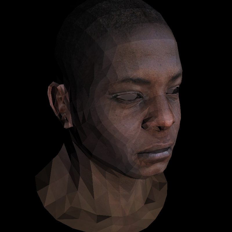
To image different perspectives of an object, imagine the camera moved in world coordinates to point $\vec{c}$, its new camera center, pointing in direction $\vec{O}$, and its orientation determined by an up direction $\vec{U}$. Take for instance the rendering below I made of an angled perspective of a bust using my software render. From a computational point-of-view the camera isn’t actually moved, rather scene points are translated and rotated to the standard frame, the one used to derive the intrinsic camera matrix. In the standard frame the camera center is $\vec{0} \in \mathbb{R}^3$, $\vec{U} = (0,1,0)$, and $\vec{O}=(0,0,-1)$ just like in Figure #2.
Suppse the camera is already located at $\vec{c} \in \mathbb{R}^3$, and oriented by $\vec{U}$ and $\vec{O}$. Moving the scene is an affine transformation $Ax + b$, where $A$ is a $3 \times 3$ matrix and $x, \ b \in \mathbb{R}^3$, which moves the camera back to the origin and reorients the camera to the standard frame. $b = -A\vec{c}$ moves the camera center to the origin and $A \in SO(3)$ reorients the camera to the standard frame; furthermore, $A$ must be a rotation matrix, because the scene shouldn’t be distorted.
Rotation and translation can be expressed together in a single a projective linear transformation. Rotation is linear but translation is not, however doing the translation in projective space is linear. Keenan Crane has a nice lecture from his computer graphics course where he visualizes translation in the plane as shearing in 3D. Anyway, this a known starting point in algebraic geometry where affine transformations are expressed as projective linear transformations like so
\[\begin{bmatrix} A & b\\ 0 & 1\\ \end{bmatrix} \begin{bmatrix} x \\ 1 \\ \end{bmatrix} \\ = \begin{bmatrix} Ax +b \\ 1 \\ \end{bmatrix} \\ .\]Constructing the Rotation Matrix
A brief digression on how to construct $A$. First construct $\vec{v}$ so that ${\vec{v}, \vec{U}, \vec{O}}$ is an orthonormal frame. Assume without loss of generality $\vec{U}$ is unit length and orthogonal; if not take $\vec{U} - \vec{O}\cdot \vec{U}$ and normalize it. Let $\vec{v} = \vec{O} \times \vec{U}$ then normalize it. The result is an orthonormal frame where $\vec{O}$ is one of the axes. Then define
\[A = \begin{bmatrix} \vec{U} \\ \vec{v} \\ -\vec{O} \\ \end{bmatrix}.\]$A$ sends $\vec{O}$ to $A \vec{O} = (0,0,-1)$ the standard optical direction, and $A$ sends $\vec{U}$ to $A \vec{U} = (1,0,0)$ the standard up direction, and finally $\vec{v}$ is mapped to $A \vec{v} = (0,1,0)$ the $y$-axis. $A$ is the desired rotation.
The Camera Matrix
With the needed rotation $A$ in hand, the affine transformation expressed as a 3D projective linear transformation is
\[\begin{bmatrix} R \ |\ t \end{bmatrix} = \begin{bmatrix} U_x & U_y & U_z & -b_x \\ v_x & v_y & v_z & -b_y \\ -O_x & -O_y & -O_z & -b_z \\ 0 & 0 & 0 & 1 \\ \end{bmatrix}.\]Finally, the full camera projection matrix is
\[\begin{align} C & = \underbrace{K}_{\text{intrinsic}} \cdot \underbrace{ \begin{bmatrix} R \ |\ t \end{bmatrix}}_{\text{extrinsic}} \\ & = \begin{bmatrix} f_v & s & c_v & 0 \\ 0 & f_u & c_u & 0 \\ 0 & 0 & 1 & 0 \\ \end{bmatrix} \begin{bmatrix} U_x & U_y & U_z & -b_x \\ v_x & v_y & v_z & -b_y \\ -O_x & -O_y & -O_z & -b_z \\ 0 & 0 & 0 & 1 \\ \end{bmatrix}. \\ \end{align}\]$C$ projects a scene in front of a camera to a rectified image expressed in $(v,u)$ image sensor coordinates.