Rotating Homogeneous Polynomials & Representations of $SO(3)$

Under the guise of rotating solid spherical harmonic functions, I want to investigate the computational aspects of representing rotations of homogeneous polynomials. The connection being that harmonic homogeneous polynomials are solid spherical harmonics. My goal in this note is to rotate solid homogeneous polynomials ( in variables $x$, $y$, and $z$ ) by computing representations of $SO(3)$ on ${\mathcal{P}}_d$, homogeneous polynomials of degree $d$. One nice aspect of computing representations of $SO(3)$ is that only algebra is required. Differential equations typically used to describe/derive spherical harmonics make no appearance in what follows.

Go straight to the code if your primary interest is the implementation of rotating homogeneous polynomials.

Preliminaries

The type of homogeneous polynomials I want to focus on are functions of the form

$SO(3)$, the group of $3-$dimensional rotations, acts on ${\mathcal{P}}_d$ by rotating coordinates of the domain ${\mathbb{R}}^3$. Suppose $p\in {\mathcal{P}}_d$ is a homogeneous polynomial then the action of $A\in SO(3)$ is

The result of the action is just another homogeneous polynomial of degree $d$, because rotations preserve distance.

Let $A,B\in SO(3)$ and denote the action instead by $\rho$. The action is actually a homomorphism.

Individually, each ${\rho }_A$ is linear.

Additionally, $A\in SO(3)$ is a change of coordinates (and therefore a linear isomorphism of ${\mathbb{R}}^3$) implies each ${\rho }_A$ has trivial kernel. To see this let $\tilde{x}=A\overrightarrow{x}$ denote the new coordinates of ${\mathbb{R}}^3$. Then $0=p(\tilde{x})\mathrm{\forall }\tilde{x}\in {\mathbb{R}}^3$ directly implies that $p=0$. With that ${\rho }_d$ is a representation of $SO(3)$ on ${\mathcal{P}}_d$. Specifically, ${\rho }_d$ is a homomorphism

What I did recently was compute the eigenvalues of $z$-axis rotations on $P_2$. All $z$-axis rotations have the following form

For notational simplicity I prefer to use $a$ and $b$ instead of $\cos \theta$ and $\sin \theta$ to describe $g_{\theta }$.

First consider representations of $A_{\theta }$ on $P_1$. The basis functions $\{x,y,z\}$ are just the coordinates functions of ${\mathbb{R}}^3$, so computing the rotated basis of $P_1$, in terms of $\{x,y,z\}$, requires simply applying $A_{\theta }$.

So for polynomial $c_{1}x+c_{2}y+c_{3}z\in P_1$ which in vector form is $\left[\begin{array}{ccc}{c}_1& c_2& c_3\end{array}\right]$

Restricting to the vector representation of $P_1$ one sees that ${\rho }_{A_{\theta }}=A_{\theta }$. Now, that the form of $\rho$ is known for $z$-axis rotations on $P_1$ the eigenvalues of the representation are easily computed. They are namely $\{e^{-i\theta },1,e^{i\theta }\}$.

To make the calculation of the representation of $A_{\theta }$ on $P_2$ easier I choose the basis to be

It’s immediately apparent that the last three basis elements are products of $z$ and the basis of $P_1$. Since the action of $A_{\theta }$ on $z$ is the identity, the representation of $A_{\theta }$ on $z{P}_1$ is the same as on $P_1$. Rewriting the $P_2$ basis with the $z{P}_1$ subspace

What might be less apparent is that the complement subspace is closed under the action of $A_{\theta }$.

Since $x^2+y^2$ is unchanged by $z-axis$ rotations, $A_{\theta }\cdot x^2+y^2=x^2+y^2.$

Therefore, the representation of $A_{\theta }$ on $P_2$ is

After substituting $a=\cos \theta$ and $b=\sin \theta$, the eigenvalues of $\rho (A_{\theta })$ are easily computed, to be $\{e^{-i2\theta },e^{-i\theta },1,e^{i\theta },e^{i2\theta }\}$. All the eigenvalues except for $1$ have multiplicity one; eigenvalue $1$ has multiplicity two.

Nice…but computing the representation of $A_{\theta }$ on ${\mathcal{P}}_1$ and ${\mathcal{P}}_2$ as I have above is not scalable at all, because there are so many terms to multiply. What I want is to express a $SO(3)$ representation in ${\mathcal{P}}_d$ for any $d$ as a product of matrices involving, necessarily, $A_{\theta }$.

Computing the Representation of $A_{\theta }$ on ${\mathcal{P}}_d$

While developing the formula for ${\rho }_2$, shown at the end of the previous section, the upper summand of ${\rho }_2$

looked to me like a sort of square of $A_{\theta }$. Indeed the portion of ${\mathcal{P}}_2$ transformed by it are the quadratic polynomials in $x$ and $y$, and the spectrum of the upper summand is a square of all the eigenvalues of $A_{\theta }$. ${\rho }_2$ is not the square of $A_{\theta }$, but the idea of somehow realizing ${\rho }_2$ as a product of $A$ with itself stuck with me. But what type of product? What properties should it preserve?

Well, the product should mimic the action of $A$ (for brevity I am dropping the subscript $\theta$) on the homogeneous basis polynomials…clearly. Consider

$A$ distributes to $x$ and $y$ in the first line. The actions of $A$ on $x$ and $y$, linear homogeneous polynomials, are resolved, resulting in a factored expression, which is expanded in the last line. The expansion is determined by the rules of multiplication: multiplication distributes over addition. So, two things are happening here. First the action of $A$ on $xy$ is actually a product of $A$-actions on lower degree homogeneous polynomials, here $x$ and $y$. Think recursion. Second, expanding the product of the actions on the lower degree factors expresses the result in the basis of ${\mathcal{P}}_2$ and relies only on the bilinearity of multiplication. Cutting to the chase…the tensor product of linear operators does both these things.

$A$ can be tensored with itself, which is a well defined extension of $A$ to ${\mathcal{P}}_1\otimes {\mathcal{P}}_1$. Identifying for the moment $xy$ with $x\otimes y$ – more on embedding ${\mathcal{P}}_1$ into tensor space ${\mathcal{P}}_1\otimes {\mathcal{P}}_1$ later – notice that the action of $A\otimes A$ on $x\otimes y$ is very close in appearance to the action of $A$ on $xy$.

$A\otimes A$, in the first line above, factors into actions of $A$ on lower degree homogeneous polynomials in each tensor coordinate: $A\cdot x$ on the left side of the tensor, and $A\cdot y$ on the right of $\otimes$. The action of $A$ on the lower degree factors is no different than before, and neither is the expansion of the factored expression in line 2 because $\otimes$ is bilinear. What remains is to collect like terms and project ${\mathcal{P}}_1\otimes {\mathcal{P}}_1$ into ${\mathcal{P}}_2$, arriving at a finally expression of the action on $xy$ in terms of ${\mathcal{P}}_2$.

Now a approach to computing ${\rho }_d$ can be stated, and it is simply

and for any degree $d$ the recursive formula

$E_d:{\mathcal{P}}_d⟶{\mathcal{P}}_1\otimes {\mathcal{P}}_{d-1}$ and $S_d:{\mathcal{P}}_1\otimes {\mathcal{P}}_{d-1}⟶{\mathcal{P}}_d$ are the embedding and projection operators, respectively. I will describe their constructions shortly in the next sections. The key though to scalably computing ${\rho }_2$ is the matrix tensor product. It is a pure matrix operation so it is easily computed/programmed.

Ordering the Basis of ${\mathcal{P}}_d$

The main function of $S_d$, the projection operator introduced in the recursive formula at the end of the previous section, is to collect the contributions of like terms. Projecting ${\mathcal{P}}_1\otimes {\mathcal{P}}_{d-1}$ into ${\mathcal{P}}_d$ accomplishes this. But what are like terms? Of main interest here are the basis elements of ${\mathcal{P}}_1\otimes {\mathcal{P}}_{d-1}$. Referring to the action of $A\otimes A$ on $x\otimes y$, it seems sensible that $x\otimes y$ and $y\otimes x$ should be considered alike.

Let basis tensors be equivalent if the sum of degrees in each variable $x$, $y$, $z$ over both tensor coordinates are the same. For clarity represent the degree sums in coordinates $(de{g}_x,de{g}_y,de{g}_z)$. A basis tensor of ${\mathcal{P}}_1\otimes {\mathcal{P}}_{d-1}$ is simply a factorization of some degree $d$ homogeneous monomial into degree $1$ and degree $d-1$ monomials; and all I am saying is that basis tensors are alike if they are factorizations of the same degree $d$ homogeneous monomial. Consider three basis tensors of ${\mathcal{P}}_1\otimes {\mathcal{P}}_{d-1}$:

All have the same degree sums coordinate; so $x\otimes x^{a-1}{y}^b{z}^c$, $y\otimes x^a{y}^{b-1}{z}^c$, and $z\otimes x^a{y}^b{z}^{c-1}$ are all equivalent. With an equivalence in hand a minimal definition of $S_d$ can be stated: $S_d$ maps tensors into their equivalence classes; specifically, $S_d$ maps ${\mathcal{P}}_1\otimes {\mathcal{P}}_{d-1}$ into ${\mathcal{P}}_1\otimes {\mathcal{P}}_{d-1}/\sim$ like so

Projecting tensors into their equivalence classes is a linear map which has the effect of collecting the contributions of equivalent terms. Take for instance a linear combination of the equivalent terms, then

The quotient space ${\mathcal{P}}_1\otimes {\mathcal{P}}_{d-1}/\sim$ is actually isomorphic to ${\mathcal{P}}_d$ via the degree sums coordinate mapping. The degree sums coordinate, $(a,b,c)$, represents a unique homogeneous monomial $x^a{y}^b{z}^c\in {\mathcal{P}}_d$; so projecting a linear combination of equivalent terms is also

The embedding operator is a sort of inverse of projection, and actually with appropriate bases ordering it is a right inverse of the projection. It doesn’t have to be though; here is a minimal defintion: it takes a given homogeneous monomial in ${\mathcal{P}}_d$ to a distinguished basis tensor among those in ${\mathcal{P}}_1\otimes {\mathcal{P}}_{d-1}$ which share the same degree sums coordinate as it. This distinguished basis tensor is an equivalence class representative of the basis tensors that project to given degree $d$ homogeneous monomial.

To realize the embedding and projection operators as matrices requires fixing the equivalence class representatives of ${\mathcal{P}}_1\otimes {\mathcal{P}}_{d-1}$, and ordering both ${\mathcal{P}}_1\otimes {\mathcal{P}}_{d-1}$ and ${\mathcal{P}}_d$. I could be idiosyncratic and choose class representatives by making some random choices; however that wouldn’t necessarily be scalable or easily scalable. Because recursion would then require storing or preserving the representatives of lower degree objects. Anyway, it’s way easier to just fix an order on ${\mathcal{P}}_d$, extend it to ${\mathcal{P}}_1\otimes {\mathcal{P}}_{d-1}$, and then choose the class representatives in the quotient object based on said order. The later is most important for creating the matrix form of the embedding; since $S_d$ collects contributions of all terms in an equivalence class, all that matters is the ordering of the bases.

The convention I use in plain words is to abstract $d$-degree homogeneous monomials into a coordinate representation $(de{g}_x,de{g}_y,de{g}_z)$, and then order the monomials first by $de{g}_z$ and then $de{g}_y$. For example the basis of ${\mathcal{P}}_2$ in ascending order is

One of the benefits of the ordering is the basis of subspace $z{\mathcal{P}}_1$, shown above in yellow, is ordered consecutively at the end; in general the pure homogeneous polynomials of degree $d$ in $x$ and $y$ are ordered before $z{\mathcal{P}}_{d-1}$. A direct consequence is that ${\rho }_d$ has a nice clear direct sum of matrices structure. ${\mathcal{P}}_1\otimes {\mathcal{P}}_{d-1}$ is ordered by coordinate, left to right; below the basis of ${\mathcal{P}}_1\otimes {\mathcal{P}}_2$ is shown in ascending order.

The degree sum coordinate of each basis tensor is written into the column on the right, and these sums aid in identifying equivalent basis tensors. For instance I have highlighted in orange every occurrence of $(1,1,1)$. The corresponding basis tensors are underlined or boxed and belong to the same equivalence class. The boxed tensor, $z\otimes xy$, is maximum element of the class. There are other equivalence classes, and each has a maximum element with respect to the defined ordering. This holds in general, so I define the equivalence class representative to be the maximum tensor among those in the class.

Projecting ${\mathcal{P}}_1\otimes {\mathcal{P}}_{d-1}$ into ${\mathcal{P}}_d$ AND Embedding ${\mathcal{P}}_d$ in ${\mathcal{P}}_1\otimes {\mathcal{P}}_{d-1}$

The embedding and projection matrices need ordered bases to be defined and constructed. Invoking the just described orderings of ${\mathcal{P}}_1\otimes {\mathcal{P}}_{d-1}$ and ${\mathcal{P}}_d$ in the previous section, create a table where:

• The row labels are basis elements of ${\mathcal{P}}_1\otimes {\mathcal{P}}_{d-1}$ listed in ascending order.
• The column labels are basis elements of ${\mathcal{P}}_d$ listed in ascending order, from left to right.
• Each cell is assigned the degree sum in coordinates, $(de{g}_x,de{g}_y,de{g}_z)$, of the corresponding row label. The degree sum coordinates facilitate identification of equivalence classes.

Since there is a clear bijection between homogeneous monomials in ${\mathcal{P}}_d$ and their degree sum coordinates, the projection $S_d$ is completely determined by the degree sums coordinate mapping. To then determine the set of equivalent basis tensors of ${\mathcal{P}}_1\otimes {\mathcal{P}}_{d-1}$, each of which labels a unique row, that map to a given homogeneous monomial of in ${\mathcal{P}}_d$, each of which its own column, one simply matches the degree sum coordinate of the degree $d$ homogeneous monomial to those in its column. To illustrate I made a table for $d=2$ and in each column $highlighted$ repeated occurances of the corresponding degree coordinate.

$\boxed{{\displaystyle Boxed}}$ and $highlighted$ cells indicate the equivalence class representative–the class maximum. Now the matrix $S_d$ can be constructed from the table by converting table cells into scalars.

• Set all NOT highlighted cells to 0.
• Set all highlighted cells to 1.

Finally, transpose the result to get the matrix form of the projection ${\mathcal{P}}_1\otimes {\mathcal{P}}_1$ into ${\mathcal{P}}_2$.

#Project tensor space into space of homogeneous polys.
S = Matrix([1, 0, 0, 0, 0, 0, 0, 0, 0],
           [0, 1, 0, 1, 0, 0, 0, 0, 0],
           [0, 0, 0, 0, 1, 0, 0, 0, 0],
           [0, 0, 1, 0, 0, 0, 1, 0, 0],
           [0, 0, 0, 0, 0, 1, 0, 1, 0],
           [0, 0, 0, 0, 0, 0, 0, 0, 1]]).

Likewise, the embedding matrix $E_d$ can be constructed from the table by converting table cells into scalars.

• Set all NOT highlighted and NOT boxed cells to 0.
• Set all highlighted and box cells to 1.

The resulting matrix is the embedding ${\mathcal{P}}_2\hookrightarrow {\mathcal{P}}_1\otimes {\mathcal{P}}_1$.

#Embed into tensor space.
E = Matrix([
	[1, 0, 0, 0, 0, 0],
	[0, 0, 0, 0, 0, 0],
	[0, 0, 0, 0, 0, 0],
	[0, 1, 0, 0, 0, 0],
	[0, 0, 1, 0, 0, 0],
	[0, 0, 0, 0, 0, 0],
	[0, 0, 0, 1, 0, 0],
	[0, 0, 0, 0, 1, 0],
	[0, 0, 0, 0, 0, 1]]).

Putting it all together, the representation $A_{\theta }$ on ${\mathcal{P}}_2$ is

In [74]: repN = S * TensorProduct(A,A) * E

In [75]: repN
Out[75]:
Matrix([
[ a**2,        -a*b,   b**2, 0,  0, 0],
[2*a*b, a**2 - b**2, -2*a*b, 0,  0, 0],
[ b**2,         a*b,   a**2, 0,  0, 0],
[    0,           0,      0, a, -b, 0],
[    0,           0,      0, b,  a, 0],
[    0,           0,      0, 0,  0, 1]])

The degree $2$ representation computed here looks a bit different than the one computed earlier at the end of the preliminaries section because the bases are slightly different; otherwise it is correct. The code I wrote can generate the matrix representation ${\rho }_d$ for any degree $d$. For instance $d=3$

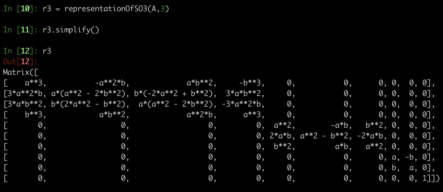
And because of the ordering ${\rho }_d$ has a nice direct sum of matrices structure…for $z$-axis rotations. The method and code I have described correctly computes representations for any 3D rotation, however no guarantees the representation will decompose nicely, as it does for $z$-axis rotations.

Eigenvalues of ${\rho }_d$

Earlier drafts of this post were actually motivated by my desire to compute the spectrum of matrix representations of $SO(3)$. Initially, I tried to avoid computing ${\rho }_d$. My hope was to use properties of $SO(3)$ and homogeneous polynomials to show that eigenvalues of a given $A\in SO(3)$ completely determine the spectrum of the representation of $A$. Anyway, I couldn’t see a way to do it, and in the meantime I developed an algorithm I spent most of this post describing to compute ${\rho }_d$. I still believe there is a way to compute the spectrum of $SO(3)$ without explicitly computing ${\rho }_d$… Update: I sort of figured out how. Most of the details are worked out in the final section.

However, since there is a recursive formula for computing ${\rho }_d$, namely

I can exploit it to make a statement about the spectrum of ${\rho }_d$. And it is this: The eigenvalues of $A\otimes {\rho }_{d-1}$, which are easy to compute, are the eigenvalues of ${\rho }_d$. Though not up to multiplicity. Clearly. ${\rho }_d$ and $A\otimes {\rho }_{d-1}$ have different shapes.

The spectrum of $A\otimes {\rho }_{d-1}$ is the product of all eigenvalues $A$ with all the eigenvalues of ${\rho }_{d-1}$. Say, $Af=\lambda f$ and ${\rho }_{d-1}g=\omega g$, then $f\otimes g$ is an eigenvector of $A\otimes {\rho }_{d-1}$ with eigenvalue $\lambda \omega$. So then to show $\lambda \omega$ is a eigenvalue of ${\rho }_d$ I can try transforming $f\otimes g$ into an eigenvector of ${\rho }_d$. Well, via the projection operator there is one candidate, $S_d(f\otimes g)$. First a technical lemma.

Lemma. A Suppose basis tensors $\beta ,\tilde{\beta }\in {\mathcal{P}}_1\otimes {\mathcal{P}}_{d-1}$ are equivalent, $\beta \sim \tilde{\beta }$. Then

1. $S_d(A\otimes {\rho }_{d-1})(\tilde{\beta }-\beta )=0$
2. ${\rho }_d{S}_d=S_d(A\otimes {\rho }_{d-1})$

Immediately one can see that 2 follows from 1; because $E_d{S}_d$ sends $\beta$ to the equivalence class representative, $E_d{S}_d\beta \sim \beta$. To understand why 1 is true, it’s best to consider how $A$ generally acts on degree $d$ homogeneous monomials, given that ${\rho }_{d-1}$ is known. Let $f_d$ be a degree $d$ homogeneous monomial; it can be factored into degree $1$ and $d-1$ monomials like $\beta$ and $\tilde{\beta }$. $A$ acts on the degree $1$ factor and ${\rho }_{d-1}$ acts on the degree $d-1$ factor, results of theses actions are simply multiplied into a single expression, and finally contributions from like degree $d$ monomial terms are collected. Multiplication is commutative and bilinear so one can take different factorizations of $f_d$ and order the operations so that the final results are the same. $S_d(A\otimes {\rho }_{d-1})$ is precisely the same procedure with the actions of $A$ and ${\rho }_{d-1}$ combined by tensor product instead of multiplication. Recall from the section above that the tensor product is bilinear, just like multiplication, though not commutative. The projection $S_d$ seen from a different perspective symmetrizes tensors, and has the effect of allowing the $x$, $y$, or $z$, in the ${\mathcal{P}}_1$ coordinate, to commute to its proper place. Therefore $S_d(A\otimes {\rho }_{d-1})$ is well defined on equivalent $\beta \in {\mathcal{P}}_1\otimes {\mathcal{P}}_{d-1}$.

With Lemma A established I can now prove that the spectrums of ${\rho }_d$ and $A\otimes {\rho }_{d-1}$ are the same.

Lemma. B $\beta \in {\mathcal{P}}_1\otimes {\mathcal{P}}_{d-1}$ is an eigenvector of $A\otimes {\rho }_{d-1}$ with eigenvalue $\lambda$ if and only if there exists $\alpha$ an eigenvector of ${\rho }_d$ with eigenvalue $\lambda$.

The implication follows directly from the matrix equality asserted in 2 of Lemma A.

In the converse direction suppose $\alpha \in {\mathcal{P}}_d$ is an eigenvector of ${\rho }_d$. Equation 2 of Lemma A and $S_d{E}_d=I_d$, the matrix identity of size $d$, imply:

• $${\rho }_d\cdot S_d{E}_d\alpha =S_d(A\otimes {\rho }_{d-1})\cdot E_d\alpha$$
• $${\rho }_d\cdot S_d{E}_d\alpha =\lambda S_d{E}_d\alpha$$

Combining shows that $\lambda$ is an eigenvalue of $A\otimes {\rho }_{d-1}$.

And there it is $A\otimes {\rho }_{d-1}$ and ${\rho }_d$ have the same spectrum,

Of course, the multiplicities will be different. But what are those multiplicities?

Dimension of the Eigenspaces: Eigenvalue Multiplicities.

From the proof of Lemma B one sees that $S_d$ projects the $\lambda -$eigenspace of $A\otimes {\rho }_{d-1}$ into the $\lambda -$eigenspace of ${\rho }_d$. Peering into the projection however is difficult because ${\rho }_{d-1}$ too has a projection component, and so on. The entire recursion has series of nested projections which hampers the analysis. Instead I can describe ${\rho }_d$ as a batch computation. And yes, there is a batch method. Which is, by the way, the definition of how $A$ acts on some monomial $p\in {\mathcal{P}}_d$: Factor $p$ into $d$ ${\mathcal{P}}_1$ factors and compute the action of $A$ on each factor. Abusing the previously introduced notation

This $S_d$ projection is a true symmetrizing operator on $\underset{i=1}{\overset{d}{⨂}}{\mathcal{P}}_1$; and just like before it projects the $\lambda -$eigenspace of $\underset{i=1}{\overset{d}{⨂}}A$ into the $\lambda -$eigenspace of ${\rho }_d$. An eigenvector of $\underset{i=1}{\overset{d}{⨂}}A$ is built from the eigenvectors of $A$ tensored $d$ times. Let $v_{-1}$, $v_0$, and $v_{+1}$ be eigenvectors of $A$ for eigenvalues $e^{-i\theta }$, 1, and $e^{+i\theta }$, respectively. Then a $\lambda -$eigenvector of $\underset{i=1}{\overset{d}{⨂}}A$ looks like

where each permutation of the elements $v_{\star }$ in the $d-$tensor is a different $\lambda -$eigenvector. Furthermore, $S_d$ sends each permutation to the same $\lambda -$eigenvector of ${\rho }_d$. What I want is to count the number of $\lambda -$eigenvectors of ${\rho }_d$, and I can build them from the $\lambda -$eigenvectors of $\underset{i=1}{\overset{d}{⨂}}A$, but I don’t have to count the permutations; I just need to count the unique combinations that produce a $\lambda -$eigenvector of ${\rho }_d$. To make counting a bit easier I represent a $e^{i\mathbf{l}\theta }-$eigenvector of $\underset{i=1}{\overset{d}{⨂}}A$ as word in $+$, $-$, and $|$ characters.

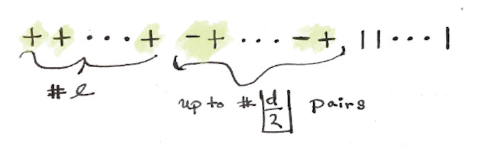
Hopefully it is clear that plus is $v_{+1}$, minus is $v_{-1}$, and pipe is $v_0$. The negative $l$ configuration would be the same drawing with the $l$ plus signs replaced with $l$ minus signs; so $e^{\pm i\mathbf{l}\theta }-$eigenspaces have the same dimension. Count the number of possible combinations like so

Therefore eigenvalues $e^{\pm il\theta }$ of ${\rho }_d$ have multiplicity

Application: Spectrum of $SO(3)$ Representation in Harmonic Polynomials

The representations of $SO(3)$ that I have described so far have been in ${\mathcal{P}}_d$, homogeneous polynomials of degree $d$. These are, however reducible representations, because degree $d$ harmonic polynomicals form a $SO(3)-$invariant subspace of ${\mathcal{P}}_d$. There is certainly more to be said about harmonic representations of $SO(3)$, but my interest right now is to use to the the dimension of the eigenspaces formula to prove degree $d$ harmonic $SO(3)$ representations have eigenvalues

and each has multiplicity one.

${\mathcal{P}}_{d+2}$ is the direct sum of degree $d$ harmonic polynomials ${\mathcal{H}}_{d+2}$ and $r^2{\mathcal{P}}_d$; so inside ${\rho }_{d+2}$ is a ${\mathcal{P}}_d$ representation, ${\rho }_d$. Then to compute the dimension of the $e^{\pm i\mathbf{l}\theta }-$eigenspaces just subtract the dimension of the $e^{\pm i\mathbf{l}\theta }-$eigenspace in ${\rho }_{d+2}$ from the dimension of the $e^{\pm i\mathbf{l}\theta }-$eigenspace in ${\rho }_d$.

When $0\le l\le d$

and when $d<l\le d+2$

Finally I have an answer/proof of Fact 1.2.1 from these Akshay Venkatesh lecture notes :)