Rotate Homogeneous Polynomials
18 Apr 2025Several years ago here on my blog I presented an algorithm for rotating homogeneous polynomials ( in variables $x$, $y$, and $z$ ) by computing representations of $SO(3)$ on $\mathcal{P}_d$, homogeneous polynomials of degree $d$. These representations are matrices in $SO(\mathcal{P}_d)$ and are rotations of $p \in \mathcal{P}_d$. While writing that post I implemented the recursive algorithm in Python, but never visually demonstrated the rotation of harmonic homogeneous polynomials by representations on $\mathcal{P}_d$. Well, I finally got around to doing just that.
On github I created a repo called rotate_spherical_harmonics. There are two scripts harmonic-dim-2-comparison.py and harmonic-dim-3-comparison.py demonstrating the effect of rotation by representations on $\mathcal{P}_2$ and $\mathcal{P}_3$, respectively, of randomly generated $SO(3)$ matrices on harmonic homogeneous polynomials:
- $xy$
- $x^2y - \frac{1}{3}y^3$
The generated figures are a visual check that the representations $\rho_d(A)$ indeed correspond to the rotations they are suppose to represent. Each figure is a side-by-side plot of a harmonic polynomial $p(x,y,z)$ in the standard x-y-z frame, and its rotation by representation $\rho_d(A)$. The colored arrows are the original and rotated frames, respectively.
On the Left ,
-
the red arrow marks the positive $z$-axis.
-
the blue arrow marks the positive $y$-axis.
-
the green arrow marks the positive $x$-axis.
Like colored arrows on the left map to like colored arrows on the right. For example, the red arrow ($z$-axis) plotted on the left is rotated by $A$ to the red arrow plotted on the right.
On the Right , is a plot of $\rho_d(A)(p)$, the rotation of $p(x,y,z)$ by $\rho_d(A)$.
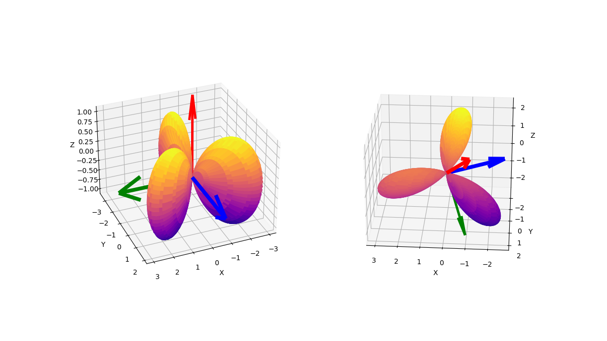
Rotate $xy$ by $\rho_2(A)$
A simple example of a harmonic polynomial is $xy$. Using script harmonic-dim-2-comparison.py a representation on $\mathcal{P}_2$ of randomly generated $SO(3)$ matrix
with axis of rotation located at $\theta = 0.7734641469345384$ radians and $\phi = 5.234991577347525$ radians, was generated and applied to harmonic homogeneous polynomial $xy$. In the figure below, $xy$ is plotted on left in the standard frame, and on the right its rotation by $\rho_d(A)$ is plotted.
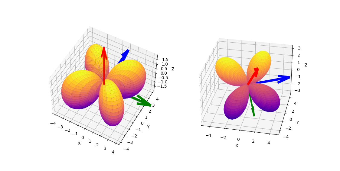
Rotate $x^2y - \frac{1}{3}y^3$ by $\rho_3(A)$
A less trivial example is harmonic polynomial $x^2y - \frac{1}{3}y^3$. Using script harmonic-dim-3-comparison.py a representation on $\mathcal{P}_3$ of randomly generated $SO(3)$ matrix
with rotation axis located at $\theta = 0.8681555864627436$ radians and $\phi = 2.0901834326555337$ radians, was generated and applied to $x^2y - \frac{1}{3}y^3$. In the figure below, $x^2y - \frac{1}{3}y^3$ is plotted on left in the standard frame, and on the right its rotation by $\rho_d(A)$ is plotted.