
Surface fairing refers to mesh smoothing and denoising. The ansatz of the paper is to cast a given mesh as a signal that can be smoothed with a low-pass filter. Furthermore, the ansatz is motivated and explained in the 1D case: Closed polygonal curves.
Given a polygon with vertices ${v_i}$, it carries functions $f: \mathbb{R}^3 \ni {v_i} \longrightarrow \mathbb{R}$, where $f(v_i) = x_i$. The function values are iterative smoothed by flowing $f$ in the scaled direction of $\Delta f $, where $\Delta$ is a discrete Laplacian. In the paper its definition is given without proof or background. \(\Delta x_i = \frac{1}{2}\Big(x_{i+1} - x_{i}\Big) + \frac{1}{2}\Big(x_{i-1} - x_{i}\Big)\)
The difference of differences around $x_i$ definition given above is an approximation of the second derivative (the 1D Laplacian). When viewing the function values at consecutive vertices as a discrete sequence, $\Delta x_i$ is essentially the second finite difference of the sequence ${x_i}$, \(\begin{align} (D^2 x)_i &= D^+(x_{i}) - D^-(x_{i-1}) \\ &= \Big(x_{i+1} - x_{i}\Big) - \Big(x_{i} - x_{i-1}\Big) \\ &= \Big(x_{i+1} - x_{i}\Big) + \Big(x_{i-1} - x_{i}\Big). \\ \end{align}\)
$D^+$ and $D^-$ are the forward and backward sequence difference operators, respectively. Yet one more interpretation can be taken from discrete curve shortening flow.
Identify the $i$-th vertex with its underlying coordinate representation, $v_i = (x_i, y_i, z_i)$. In the framework of this paper, each coordinate function ($x_i$, $y_i$, and $z_i$) is a function defined on the vertices of a polygon – in the 1-D case. Consider the picture below of $v_i$ and its 1-neighbors in a polygon.
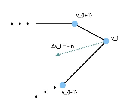
The differences $a = v_{i+1} - v_{i}$ and $b = v_{i-1} - v_{i}$ are vectors with a common base, representing neighboring segments at $v_i$, whose sum is an (approximate) inward pointing normal at $v_i$, between segments and $a$ and $b$. With each iteration vertices are moved in the direction of the inward normal (at convex points) or in the direction of the outward normal (at concave points). In this way variations in the polygonal are flattened, and the polygon as a whole shrinks to a round point – curve shortening flow. In the smooth case it is even more clear because $\Delta \gamma = \frac{d^2\gamma}{ds^2} = \kappa \vec{n}$. One of the papers contributions is a two step iteration to prevent shrinkage.
When written as a matrix the discrete Laplacian of the sequence is the circulant matrix, \(K = -\frac{1}{2}\begin{bmatrix} -2 & 1 & 0 & \cdots & 0 & 1\\ 1 & -2 & 1 & 0 & \cdots & 0 \\ 0 & 1 & \ddots & \ddots & \ddots & \vdots \\ 0 & 0 & \ddots & \ddots & 1 & 0 \\ \vdots & \vdots & \ddots & 1 & -2 & 1 \\ 1 & 0 & \cdots & 0 & 1 & -2 \\ \end{bmatrix}.\)
By the Spectral Theorem $K$ symmetric implies that it can be diagonalized by some real orthogonal matrix, $\Lambda = O K O^T$. Therefore, $K$ has real eigenvalues. Though, orthogonally diagonalizing $K$ is overkill.
Alternate proof:
Suppose $0 \neq \lambda \in \mathbb{C}$ is an eigenvalue of $K$, for some $v \in \mathbb{C}^n$. Also define the inner product on $\mathbb{C}^n$ to be $v \cdot w := v^T \bar{w}$. The product $Kv \cdot v$ can be computed two different ways:
Then, one must conclude $\bar{\lambda} = \lambda \ \Longrightarrow \lambda \in \mathbb{R}$. $\Box$
By a similar argument, it can be shown that $v \neq w$ eigenvectors of $K$, which do not span each other, must be orthogonal, if they have different eigenvalues. Just compute $Kv \cdot w$ two different ways. Assuming $\lambda_v \neq \lambda_w$ then
Since $\lambda_v \neq \lambda_w \ \Longrightarrow \ v \cdot w = 0$.
Eigenvectors of $K$ belonging to the same eigenspace are also orthogonal. For a proof checkout these notes.
$K$ is a circulant matrix so we can calculate eigenvalues. In my notes on circulant matrices, I did just that. In general the eigenvalues have the following form.
\(\begin{equation} \lambda_C = c_0 + c_1 e^{i\frac{2\pi k}{n}} + c_2 e^{i\frac{4\pi k}{n}} +\cdots + c_{n-1}e^{i\frac{2\pi k(n-1)}{n}} \end{equation}\) For $\Delta \approx K$, all coefficients $c_i$ are zero except for $c_0 = -2$, $c_1 = 1$, and $c_{n-1} = 1$. Substituting those specific coefficients into the eigenvalue formula and simplifying gives,
\[\begin{align} \lambda_k &= -2 + e^{i\frac{2\pi k}{n}} + e^{i\frac{2\pi k(n-1)}{n}} \\ &= -2 + e^{i\frac{2\pi k}{n}} + \cancelto{1}{e^{i2\pi k}} + e^{-i\frac{2\pi k}{n}} \\ &= -1 + 2\cos\big(\frac{2\pi k}{n}\big) \end{align}\]Based on the previous section, we expected the eigenvalues of $K$ to be real, and they are indeed real.
Let $p(x_1, x_2, \cdots, x_n): U \subsetneq \mathbb{R}^n \longrightarrow V \subsetneq M^n$ be local coordinates on $M^n$. Let $p_1(x_1, ) = $ \(\nabla p = \begin{bmatrix} \frac{dp_1}{dx_1} & \frac{dp_2}{dx_1} & \cdots & \frac{dp_n}{dx_2} \\ \frac{dp_1}{dx_2} & \frac{dp_2}{dx_2} & \cdots & \frac{dp_n}{dx_2} \\ \vdots & \vdots & \vdots & \vdots &\\ \frac{dp_1}{dx_n} & \frac{dp_2}{dx_n} & \cdots & \frac{dp_n}{dx_n} \\ \end{bmatrix}\) Now the Laplace-Beltrami operator \(div \nabla p = \begin{bmatrix} \frac{d}{dx_1} & \frac{d}{dx_2} & \cdots & \frac{d}{dx_n} \end{bmatrix} \begin{bmatrix} \frac{dp_1}{dx_1} & \frac{dp_2}{dx_1} & \cdots & \frac{dp_n}{dx_2} \\ \frac{dp_1}{dx_2} & \frac{dp_2}{dx_2} & \cdots & \frac{dp_n}{dx_2} \\ \vdots & \vdots & \vdots & \vdots &\\ \frac{dp_1}{dx_n} & \frac{dp_2}{dx_n} & \cdots & \frac{dp_n}{dx_n} \\ \end{bmatrix}\)