
Perspective Projection
03 Mar 2022Derivations of the perspective projection matrix, whether in books or on the web, always feel either overly complicated or completely lacking in detail–sometimes the perspective projection matrix is just stated without much explaination. In surveys of image projection, that is projection of a 3D scene to 2D, orthographic projection is presented as a contrasting method without relation to perspective projection. While the light model–how light travels to the image plane–underlying the different projection types differ, both can be formulated as projective transformations from their respective view volumes to the canonical view volume. Once in the canonical frame, $x$ and $y$ coordinates are already considered projected, which is to say they are in image plane coordinates; so both perspective projection and orthographic projection are image projections on each depth slice of their respective view volumes. When rendering to the screen, depth information is required to determine those objects and parts of objects not occluded by other objects.
At least at the level of formulas perspective projection and orthographic projection look similiar enough to believe perspective projection could be written in terms of orthographic projection, which IMHO greatly simplifies its derivation. In this note I derive the perspective projection matrix by factoring it through the orthographic view volume.
Perspective

Perspective in art and photography is about representing depth of a 3D scene in 2D. When thinking about perspective the first image that comes to mind, and it ought to be familiar to most people, is of railroad tracks running off into the distance. The tracks though parallel are rendered as angled toward each other such that they would eventually meet at some point behind the image plane called the vanishing point, or the point at infinity. Objects further away appear smaller than those closer to the eye. This is what the world looks like to us and cameras, since cameras are meant to capture the world as we see it.
In a previous post I derived the camera matrix, a projective transformation of a 3D scene in front of a camera onto an image plane behind the camera center. Indeed, camera projection renders a 3D scene in perspective on the image plane. Scene points are projected onto the image plane by what I’ll call homogenous division; that is $x$ and $y$ coordinates are divided by the depth coordinate $z$. Consequently, scene points further away are projected closer to the image center. As a result, an object in the scene which has depth (e.g. railroad tracks) will render so portions of the object further away from the camera naturally angle inward, toward the image center; therefore, objects located further away from the camera center will appear smaller. Suppose the image plane is located at $z = F$, then
\[P = \begin{bmatrix} F & 0 & 0 & 0 \\ 0 & F & 0 & 0 \\ 0 & 0 & F & 0 \\ 0 & 0 & 1 & 0 \\ \end{bmatrix}\]is a basic perspective projection and it is defined on $\mathbb{A}^3 \subsetneq \mathbb{RP}^3$, the affine space of $\mathbb{RP}^3$. In the equation on the next line $P$ acts on scene points by copying the $z$ cooridinate into the $w$ coordinate, and after homogenous division lines are projected onto the $z = F$ plane of $\mathbb{A}^3$.
\[\begin{bmatrix} F & 0 & 0 & 0 \\ 0 & F & 0 & 0 \\ 0 & 0 & F & 0 \\ 0 & 0 & 1 & 0 \\ \end{bmatrix} \begin{bmatrix} x \\ y \\ z \\ 1 \\ \end{bmatrix} = \begin{bmatrix} Fx \\ Fy \\ Fz \\ z \\ \end{bmatrix} \sim \begin{bmatrix} Fx / z \\ Fy / z\\ F \\ 1 \\ \end{bmatrix}.\]$P$ renders the entire scene in perspective on the image plane even though we humans and cameras can not perceive the whole scene. This limitation or field of view is modeled by a 3D solid region in front of the camera. Points and triangles outside the field of view are filtered out before projecting to the screen.
Filtering out points and triangles outside the view volume potentially eliminates a lot of extra work and unwanted artifacts. For instance, without a near plane the rendered output might exhibit z-fighting. Choosing the near plane so it is not too close to the eye/camera (at a distance smaller than floating point precision), and keeping the near and far plane not too far apart reduces the chance of z-fighting.
Presentations of image projection in books and course notes/videos focus on two main types of view volumes: the view frustum and the orthographic view volume.
View Frustum
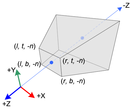
The view frustum is a pyramidal solid primarly defined by the dimensions of its near face at $z = -n$ and the location of its far face at $z = -f$. The sides are defined by projective lines through the edges of the near face. The view frustum is depicted below in Figure #1.
A basic perspective projection
\[P = \begin{bmatrix} n & 0 & 0 & 0 \\ 0 & n & 0 & 0 \\ 0 & 0 & n & 0 \\ 0 & 0 & -1 & 0 \\ \end{bmatrix}\]projects points in the frustum onto the near face, at $z=-n$, along lines through the origin. $P$ flattens the frustum onto the near face, eliminating the depth information. To facilitate $z$-buffering, an occlusion resolution technique, $P$ is later altered to, at least, preserve the relative ordering of points by depth values.
Orthrographic View Volume
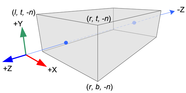
The orthrographic view volume is a cuboid solid and like the view frustum its shape is determined by the dimensions of the near face at $z=-n$ and the location of the far face at $z = -f$. It’s depicted below in Figure #2.
In contrast to the view frustum, light travels in lines perpendicular to the image plane in the orthographic view volume. Consequently, parallel lines in the scene stay parallel in the image, which is why orthographic projection is also referred to as parallel projection. There are actually many different types of parallel projections.
Let the near face be the image plane, then an orthographic projection sends points in the cuboid volume along perpendicular lines to the near face; essentially the $z$-coordiante is erased and the $x$ and $y$ coordinates are translated to the near face. When formulated as a projective matrix acting on $\mathbb{A}^3$ the just described basic orthographic projection is
\[O = \begin{bmatrix} 1 & 0 & 0 & 0 \\ 0 & 1 & 0 & 0 \\ 0 & 0 & 0 & -n \\ 0 & 0 & 0 & 1 \\ \end{bmatrix}.\]Canonical View Volume
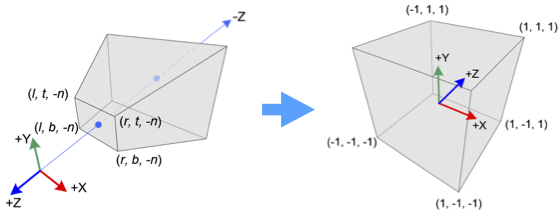
To speed the clipping proccess the given view volume, either type, is mapped to a special orthographic volume called the canonical view volume. It is a cube centered at the origin depicted in Figure #3. Mapping to a canonical view volume allows for simpler hardware. Throughout this post I use the OpenGL definition of the canonical frame.

Because the canonical volume is an orthographic volume, points in the canonical frame are projected to the screen orthographically. In the OpenGL standard the screen is located at $z = 1$.
Orthographic Projection
A projective transformation that bijectivily takes the orthographic view volume to the canonical view volume is called an orthographic projection. The orthrographic view volume is defined by planes: $z=-f$, $z=-n$, $y=t$, $y=b$, $x=l$, and $x=r$. Here $l=$left, $r=$right, $t=$top, $b=$bottom, $n=$near, and $f=$far; necessarily $r>l$, $t >b$, and $f > n$.

Since both volumes are the same shape but with different dimensions and centers, there is an affine map $O_{proj}$ which maps the orthographic volume bijectivily to the canonical volume. $O_{proj}$ translates the orthographic view center to the origin and scales all the axises so the cuboid sides are all length 2. For frameworks like OpenGL and Vulkan the camera in the target coordinate system looks down the positive $z$-axis; therefore, $O_{proj}$ must also flip the $z-$axis. Translating and scaling gives
\[\begin{align} O_{proj} &= \underbrace{ \begin{bmatrix} \frac{2}{r-l} & 0 & 0 & 0 \\ 0 & \frac{2}{t-b} & 0 & 0 \\ 0 & 0 & -\frac{2}{f-n} & 0 \\ 0 & 0 & 0 & 1 \\ \end{bmatrix} }_{\text{scaling}} \underbrace{ \begin{bmatrix} 1 & 0 & 0 & -\frac{r+l}{2} \\ 0 & 1 & 0 & -\frac{t+b}{2} \\ 0 & 0 & 1 & \frac{f+n}{2} \\ 0 & 0 & 0 & 1 \\ \end{bmatrix} }_{\text{translation}} \\ &= \begin{bmatrix} \frac{2}{r-l} & 0 & 0 & \frac{l+r}{l-r} \\ 0 & \frac{2}{t-b} & 0 & \frac{b+t}{b-t} \\ 0 & 0 & -\frac{2}{f-n} & -\frac{f+n}{f-n} \\ 0 & 0 & 0 & 1 \\ \end{bmatrix} \\ \end{align}\]the orthographic projection matrix.
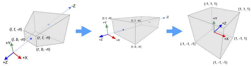
Projecting the View Frustum to the Orthographic View Volume
Consider a $yz$-cross section of the view frustum; one is drawn on the left side of Figure #4. Now, imagine collapsing the top and bottom of the view frustrum until the $yz$-cross section looks rectangular, like the right side of Figure #4. Deforming a $yz$-cross section in this way transforms lines passing through both the near face, at $z = -n$, and the origin into horizontal lines. Figure #4 depicits this deformation: The green arrow on the left side of Figure #4 is a segment of a line that passes through the origin and the near face, and it is mapped to the horizontal green arrow in the rectangle on the right.

Naturally, both green arrows intercept the near face at the same point. Which implies, the $y$-coordinate of the near face intercept is the $y$-value of the horizontal green arrow (on the right in Figure #4). Therefore, the horizontal green arrow is constructed by projecting the sloping green arrow in the view frustum section (left side of Figure #4) to the near face. Since any point in the interior of the view frustum section lies on some sloped line through the origin, the $y$-coordinate of any point in the view frustum is mapped by the deformation to its projection on the near face; specifically, if $(y,z)$ is a point in the view frustum section, then $y \mapsto \frac{-ny}{z}$ on the near face. A derivation of the projected $y$ value can be found in my previous post on camera matrices.
From Heuristic to Implememation
Because the deformation includes a projection of the $y$ coordinate, it can be conceived of as projective transformation
\[M_{pp} = \begin{bmatrix} n & 0 & 0 \\ 0 & A & B \\ 0 & -1 & 0 \end{bmatrix},\]where $A$ and $B$ are unknowns. Originally, I thought $M_{pp}$ should be the identity on $z$, but constructing a linear map which is the identity on the depth interval $-n < z < -f$ after division by $-z$ is only possible if $z$ is squared. Not a linear operation. While the deformation isn’t in general the identity on $z$, it must fix points on the near face,
\[\begin{equation} \begin{bmatrix} n & 0 & 0 \\ 0 & A & B \\ 0 & -1 & 0 \end{bmatrix} \begin{bmatrix} y \\ -n \\ 1 \\ \end{bmatrix} = \begin{bmatrix} ny \\ -n \cdot n \\ n \\ \end{bmatrix} \sim \begin{bmatrix} y \\ -n \\ 1 \\ \end{bmatrix} \end{equation}.\]It must also fix the $z$-coordinate of points on the far face,
\[\begin{equation} \begin{bmatrix} n & 0 & 0 \\ 0 & A & B \\ 0 & -1 & 0 \end{bmatrix} \begin{bmatrix} y \\ -f \\ 1 \\ \end{bmatrix} = \begin{bmatrix} ny \\ -f \cdot f \\ f \\ \end{bmatrix} \sim \begin{bmatrix} \frac{ny}{f} \\ -f \\ 1 \\ \end{bmatrix} \end{equation}.\]Both of these boundary conditions can be reduced to the system of equations
\[\begin{cases} -fA + B &= -f^2\\ -nA + B &= -n^2. \\ \end{cases}\]Solving the system, $A = n+f$ and $B=nf$.
The same derivation could have been made for the $xz$-cross section of the view frustum without any change. Indeed, $x$ values of points in the view frustum must also be projected to the near face independent of $y$ and $z$. Therefore, the deformation of the view frustum to the orthographic volume is projective transformation
\[M_{pp} = \begin{bmatrix} n & 0 & 0 & 0 \\ 0 & n & 0 & 0 \\ 0 & 0 & n+f & nf \\ 0 & 0 & -1 & 0 \\ \end{bmatrix}.\]Putting it All Together
All the pieces are in place to describe perspective projection as a product of simplier transformations. After projecting the view frustum to the orthographic view volume and applying orthographic projection, the full perspective projection matrix is
\[\begin{align} P_{proj} &= O_{proj} M_{pp} \\ &= \begin{bmatrix} \frac{2}{r-l} & 0 & 0 & \frac{l+r}{l-r} \\ 0 & \frac{2}{t-b}& 0 & \frac{b+t}{b-t} \\ 0 & 0 & -\frac{2}{f-n} & -\frac{f+n}{f-n} \\ 0 & 0 & 0 & 1 \\ \end{bmatrix} \begin{bmatrix} n & 0 & 0 & 0 \\ 0 & n & 0 & 0 \\ 0 & 0 & n+f & nf \\ 0 & 0 & -1 & 0 \\ \end{bmatrix}\\ &= \begin{bmatrix} \frac{2n}{r-l} & 0 & \frac{r+l}{r-l} & 0 \\ 0 & \frac{2n}{t-b}& \frac{t+b}{t-b} & 0 \\ 0 & 0 & \frac{n+f}{n-f} & \frac{2nf}{n-f} \\ 0 & 0 & -1 & 0 \\ \end{bmatrix}. \end{align}\]Though not at all necessary I carried out these calculations in a Juypter notebook.